The Peano Curve · Fractal Fair

The first published space-filling curve — a 1-D line whose image is a full 2-D square.

History

In 1890, Giuseppe Peano shocked the mathematical world with a construction nobody thought possible: a continuous curve passing through every point of a filled square. Until then, “curve” and “one-dimensional” were treated as nearly synonymous.

Anecdote

Peano’s original paper contained no illustrations at all — just equations. The now-familiar boustrophedon (“as the ox turns”) picture was supplied later by other mathematicians trying to visualise what Peano had only proven.

Construction

Peano’s curve is an L-system, in the same spirit as the L-Systems chapter: axiom L, with L and R each expanding one segment into nine, sweeping a 3×3 grid in a boustrophedon (back-and-forth, like an ox ploughing a field) pattern, angle 90°. Before looking at the full rule, it’s worth watching what the very first rewrite actually draws.

Applying rule $L$ once to the axiom L gives LFRFL-F-RFLFR+F+LFRFL. Stripping out the non-drawing Ls and Rs, the turtle sees: forward, forward, turn right, forward, turn right, forward, forward, turn left, forward, turn left, forward, forward — eight segments sweeping back and forth across three rows, a miniature version of the same boustrophedon pattern the full curve uses at every scale:

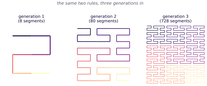
Generations 1 through 3 of the Peano curve build-up — The same two rules, three generations in. Nine segments become a scaled copy of the whole pattern at every step, which is why the segment count multiplies by 9 each generation rather than Hilbert’s 4.

Now the full rule set:

L \to LFRFL{-}F{-}RFLFR{+}F{+}LFRFL, \qquad R \to RFLFR{+}F{+}LFRFL{-}F{-}RFLFR

Because each step multiplies the segment count by $9=3^2$ : $D = \log 9/\log 3 = 2$ — the curve’s image, in the limit, is the entire filled square.

★Cool Fact

A space-filling curve is necessarily not injective: some points are visited more than once. A continuous map from a line onto a plane cannot be one-to-one, so self-intersection is a mathematical necessity, not a flaw.

Python implementation

Pseudocode first

Algorithm in one glance Rewrite

Rules plus a shared turtle

peano(n) {
    word = rewrite("L", PEANO_RULES, n)
    return turtle(word, angle=90)
}

The executable version keeps the same shape; shared plotting/export details live in fractalfair_helpers.py.

def peano(iterations=3):
    word = rewrite(AXIOM, RULES, iterations)
    return np.array(turtle_segments(word, 90))

λThe Same Idea in Haskell

rules = M.fromList
  [ ('L', "LFRFL-F-RFLFR+F+LFRFL")
  , ('R', "RFLFR+F+LFRFL-F-RFLFR") ]

peanoDiagram iterations = mconcat
  [ fromVertices [p0, p1] # lc (fireGradient ...) | (p0, p1) <- segs ]
  where segs = turtleSegments (rewrite rules "L" iterations) 90 0 1.0

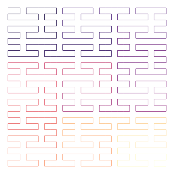
Order-3 Peano curve — **Figure:** 729 unit segments sweeping every cell of a 27×27 grid in one continuous path.