The Mandelbrot Set
The index of every Julia set at once — and the most recognisable image in popular mathematics.
History
Benoit Mandelbrot, at IBM, first generated crude printer plots of the set that now bears his name in 1978–1980, building on Fatou and Julia’s earlier work. Higher-resolution images by Heinz-Otto Peitgen and Peter Richter through the early 1980s turned the set into an unlikely public sensation. The name itself was coined not by Mandelbrot but by Adrien Douady and John Hubbard, in his honour.
The earliest computer plots, run on IBM line printers in the late 1970s, were so low-resolution that Mandelbrot initially suspected the fuzzy structures near the boundary were printer artefacts. Higher-resolution runs confirmed the “fuzz” was real: infinitely intricate structure, all the way down.
Construction
Pick a point in the complex plane, and iterate the same rule as the Julia chapter — but starting from every time, with itself now the thing that varies from pixel to pixel:
Two concrete examples before the formal definition. Take : every iterate is , forever — bounded, so is in the set. Now take : , , , — clearly diverging, so is outside the set. The Mandelbrot set is exactly the collection of every that behaves like the first example rather than the second:
If ever exceeds 2, the orbit is guaranteed to diverge — so every renderer iterates until (colour by how long that took) or a generous cap (colour it black — presumed in the set). The Fatou–Julia theorem: the filled Julia set is connected iff — which is why the Mandelbrot set can be read as an index of every Julia set at once, one point per parameter .
The Mandelbrot set’s boundary has Hausdorff dimension exactly 2 (Shishikura, 1991) despite the set itself having finite area (≈ 1.5065918, no known closed form). A boundary that is simultaneously a curve and fully two-dimensional is possible only because it’s a fractal.
ORBIT LAB
One pixel, one orbit
Choose c, then watch z₀=0 march under z ← z²+c. The full Mandelbrot image is this experiment repeated for every pixel.
The dashed circle is |z|=2. Once an iterate crosses it, escape is guaranteed.
From one orbit to the whole parameter plane
Every pixel in the famous image is a tiny dynamical experiment. Dark points survive the iteration cap; coloured points escape, and their colour records how quickly. The boundary is where nearby parameters can have radically different fates.
LINKED EXPLORER
Mandelbrot chooses the parameter; Julia reveals its world
Click anywhere in the Mandelbrot plane. That point becomes c in z ← z² + c, and the Julia set on the right is redrawn immediately.
The right-hand picture answers a different question with the same recurrence. Pick a parameter in the Mandelbrot plane, then inspect the entire world of starting points for that fixed parameter. This is the most useful way to feel the Fatou–Julia connection before meeting its theorem.
Python implementation
Pseudocode first
for each pixel c {
    z = 0
    repeat until |z| > 2 or the limit is reached
        z = z*z + c
    colour c by escape time
}
The executable version keeps the same shape; shared plotting/export details live in fractalfair_helpers.py.
c = grid_of_parameters()
z = np.zeros_like(c)
for i in range(max_iter):
    z[alive] = z[alive]**2 + c[alive]
    escaped = alive & (abs(z) > 2)
    time[escaped] = i + 1
    alive &= ~escaped
escapeTime :: Int -> Complex Double -> Double
escapeTime maxIter c = go 0 0
  where
    go n z | n >= maxIter    = 0
           | magnitude z > 2 = fromIntegral n / fromIntegral maxIter
           | otherwise       = go (n+1) (z*z + c)
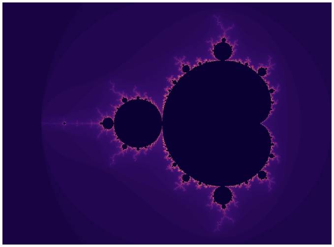
Figure: Coloured by smoothed escape time on a fire palette; the set itself is rendered black. Every bulb sprouts infinitely many smaller bulbs and filaments.
Bottomless wonders spring from simple rules, repeated without end.
Beyond its role as the most recognisable image in popular mathematics, the Mandelbrot set is a standard teaching example for parameter-space bifurcation structure, and its rendering algorithm is a perennial benchmark for GPU programming and parallel computing frameworks.