The Newton Fractal · Fractal Fair

A local, deterministic root-finder — yet the global picture of which root it converges to is a fractal.

History

Newton’s method is three centuries old — he described it in 1669, though it wasn’t published until 1711, in De analysi per aequationes numero terminorum infinitas. Applied to a real function, it’s a purely local, one-root-at-a-time procedure: start near a root, follow the tangent line down to where it crosses zero, repeat. Nothing about that process suggests a fractal.

The fractal appears once you ask a different, global question: given a complex polynomial with several roots, colour every possible starting point $z_0$ by which root the iteration eventually converges to. Arthur Cayley posed exactly this question in 1879 for quadratics and cubics, correctly solving the quadratic case — the plane splits cleanly into two halves — but flagging the cubic as far harder. It is: with three or more roots to choose between, the boundary separating one basin from another turns out to be fractal, since it must simultaneously border every other basin at once.

Anecdote

Cayley’s 1879 note ends by admitting he couldn’t complete the analysis for cubics. It would be more than a century before anyone could — not because the mathematics was missing, but because nobody could yet render millions of iterated points fast enough to see what he was asking about.

FROM CALCULUS TO FRACTALS

First watch ordinary Newton iteration

Before colouring millions of starting points, follow just one. For f(x)=x³−1, draw the tangent at xₙ; where that tangent meets the x-axis becomes xₙ₊₁.

x₀ = 1.8000Click “Take one Newton step”.

Once we move from the real line to the complex plane, a polynomial can have several roots. Asking which root wins from each starting point? turns this familiar tangent method into the coloured basins of the Newton fractal.

Construction

z_{n+1} = z_n - \frac{p(z_n)}{p'(z_n)}, \qquad p(z) = z^3 - 1

Colour every $z_0$ by which of the three cube roots of unity the iteration converges to. Near each root, convergence is smooth and classical; along the basin boundaries, the picture is fractal.

★Cool Fact

The three basins for $z^3-1$ meet at every point of their common boundary — no point on the boundary between “red” and “blue” isn’t also arbitrarily close to “green.” This Lakes-of-Wada property was a theoretical curiosity for seven decades before Newton fractals turned out to be full of naturally occurring examples.

Python implementation

Pseudocode first

Algorithm in one glance Iterative

Follow Newton to a root

for each starting point z {
    repeat until z reaches a root
        z = z - (z^3-1)/(3z^2)
    colour by the winning root
}

The executable version keeps the same shape; shared plotting/export details live in fractalfair_helpers.py.

def step(z):
    return z - (z**3 - 1)/(3*z**2)

for i in range(max_iter):
    z = step(z)
    # mark newly converged points; later colour by nearest root

λThe Same Idea in Haskell

converge :: Int -> Complex Double -> (Int, Int)
converge maxIter = go 0
  where
    go n z
      | n >= maxIter                   = (nearestRootIx z, n)
      | any (\r -> magnitude (z-r) < 1e-6) roots
                                        = (nearestRootIx z, n)
      | otherwise                      = go (n+1) (newtonStep z)

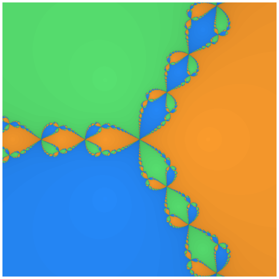
Newton fractal for z^3-1 — **Figure:** Orange, blue, and green mark the three basins of attraction, shaded darker where convergence took longer.

Where You've Seen This

The basin structure is used pedagogically throughout numerical analysis and dynamical systems courses as the canonical example of sensitive dependence on initial conditions in an otherwise completely deterministic algorithm.