The Barnsley Fern
Four affine maps and a handful of probabilities encode something that looks uncannily like a real frond.
History
Michael Barnsley published his fern in 1988 in Fractals Everywhere as the flagship demonstration of Iterated Function Systems applied to natural forms. Unlike the earlier fractals in this book, the fern was designed from the start as a computer-graphics object: a vivid demonstration that a handful of numbers could encode something as organically complex as black spleenwort.
Barnsley’s real motivation was compression. If a recognisable fern can be encoded in under thirty numbers rather than millions of pixels, perhaps whole photographs could be too. This idea grew into fractal image compression, commercialised in the early 1990s before more conventional codecs won out on speed.
Construction
Each of the four maps below is an affine transformation — a linear stretch-and-rotate given by , plus a shift given by , exactly the family of maps shown in Chapter 0’s “original / translated / scaled / rotated / affine” figure, just with four different specific choices of numbers:
The chaos game is the same idea used for the Sierpinski triangle, generalised from “jump toward a random vertex” to “apply a random map”: start anywhere, at every step pick one of the four maps below — weighted by its probability , so the frond gets picked far more often than the stem — apply it, plot the new point, and repeat tens of thousands of times.
Before the matrix: grow the stem by hand
The Stem rule is the gentlest possible affine map. Forget matrices for a moment and read two instructions:
Start at . The new -coordinate is forced to zero, while the height becomes only sixteen percent of what it was:
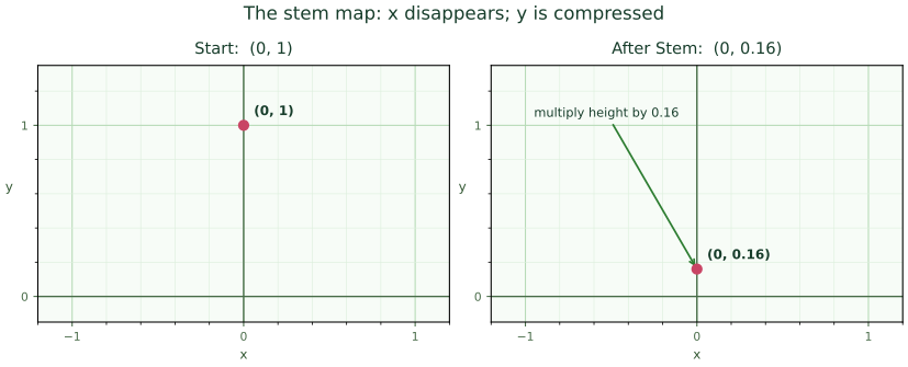
Figure: The graph has major lines one unit apart. You can literally locate , then see the Stem rule move it down the same -axis to .
Aha: the Stem map is not “drawing a line.” It is repeatedly collapsing the whole plane onto the vertical axis and compressing height. Even would become : the old is simply discarded.
Apply it again and the height is ; once more gives . The repeated rule squeezes points toward the base of the stem.
Now grow the main frond, one point at a time
The dominant rule is
Read this first as a sentence, not a matrix:
keep most of the old position → tilt a little → move upward by 1.6.
Starting at :
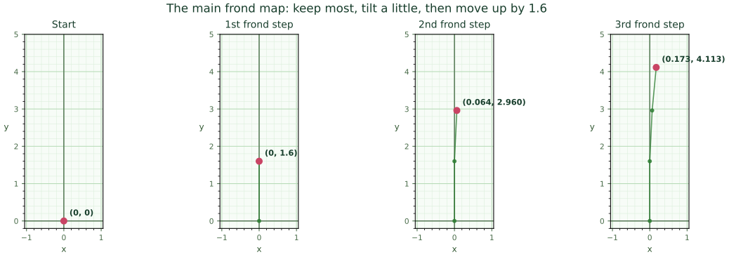
Figure: The axes and unit grid do not move between panels. The large effect is the repeated upward translation; the small cross-terms create the gentle sideways drift.
Now the coefficients have something to attach to in your mind: means “keep most,” the tiny terms create a slight tilt, and lifts the new copy upward.
Only now compress the story into a matrix
The matrix is not new mathematics; it is simply a compact container for the two coordinate instructions you have already followed by hand.
| Map | a | b | c | d | e | f | p |
|---|---|---|---|---|---|---|---|
| Stem | 0.00 | 0.00 | 0.00 | 0.16 | 0.00 | 0.00 | 0.01 |
| Frond | 0.85 | 0.04 | −0.04 | 0.85 | 0.00 | 1.60 | 0.85 |
| Left leaflet | 0.20 | −0.26 | 0.23 | 0.22 | 0.00 | 1.60 | 0.07 |
| Right leaflet | −0.15 | 0.28 | 0.26 | 0.24 | 0.00 | 0.44 | 0.07 |
Because each map has its own probability, the point density isn’t uniform: it’s denser near the main stem and sparser near the leaflet tips, matching how a real frond thickens toward its spine.
Experiment: geometry versus probability
Here is a subtle distinction worth seeing rather than merely reading. Keep the same four affine maps, but change how often each one is selected. The geometric IFS attractor is determined by the maps; the probabilities determine how a random orbit samples that attractor — its invariant measure.
This is why “random” does not mean “formless.” In the Sierpinski game, equal probabilities make the sampling visually even. In the fern, unequal probabilities are part of the visual story: the 85% frond map makes the orbit spend most of its time building the long recursive backbone, while the rarer maps repeatedly kick it into the side leaflets.
Python implementation
Pseudocode first
fern(n) {
    p = (0,0)
    repeat n times {
        map = choose one affine map using its probability
        p = map(p)
        emit p
    }
}
The executable version keeps the same shape; shared plotting/export details live in fractalfair_helpers.py.
def fern(n=140_000, seed=3):
    rng = np.random.default_rng(seed)
    p, points = np.zeros(2), np.empty((n,2))
    for i in range(n):
        a,b,c,d,e,f,_ = MAPS[rng.choice(4, p=MAPS[:,6])]
        x,y = p
        p = [a*x+b*y+e, c*x+d*y+f]
        points[i] = p
    return points
pick :: StdGen -> (AffineMap, StdGen)
pick g = (go fernMaps u, g')
  where
    (u, g') = randomR (0, 1 :: Double) g
    go (mp:rest) r | r <= amP mp = mp
                    | otherwise   = go rest (r - amP mp)
    go [] _ = last fernMaps
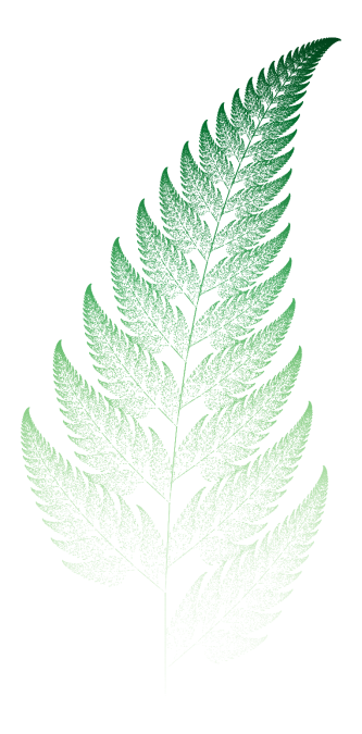
Figure: 140,000 points, shaded from pale (stem) to deep green (tips). Every sub-frond is a smaller copy of the whole.
IFS-style procedural generation in the spirit of the fern is used today in games and graphics to generate foliage, terrain detail, and other organic content on the fly from a small parameter set.