Introduction to Fractals
What fractals actually are, the century of mathematicians who discovered them piece by piece, and the three distinct mechanisms — IFS, L-systems, and escape-time iteration — every chapter that follows is built from.
In 1975 Benoit Mandelbrot needed a word for a class of shapes that classical geometry had mostly ignored: sets that are too irregular for the smooth lines and circles of Euclid, yet not merely “random noise” either — shapes with structure at every scale. He coined fractal from the Latin fractus, meaning broken or fractured. The name stuck; so did the idea. This page is a short tour of what that idea actually is, who spent the better part of a century discovering pieces of it before Mandelbrot named the whole, and the three distinct mechanisms every fractal on this site is built from.
What is a fractal?
Most of the objects on this site share one property: zoom in, and you see (an approximate or exact copy of) the whole again. A branch of a fern looks like a small fern; a piece of a coastline looks like a small coastline; a tiny corner of the Mandelbrot set contains a distorted copy of the entire set. This property is called self-similarity, and it comes in two flavours worth distinguishing from the start:
- Exact self-similarity, produced by an Iterated Function System or an L-system: the whole is a union of smaller, exact (if rotated or reflected) copies of itself.
- Quasi self-similarity, where zoomed-in copies are similar but not identical to the whole — the hallmark of the escape-time fractals later in this site.
Ordinary curves are one-dimensional and ordinary surfaces are two-dimensional — but fractal boundaries often behave as though they have a dimension strictly between the two. For self-similar sets, the similarity dimension makes this precise: if a shape is built from copies of itself, each scaled down by a factor , its dimension is
The Koch curve is built from copies scaled by , giving — a curve that is “more than a line but less than a plane.”
Mandelbrot’s very first fractal-adjacent question, posed in a 1967 Science paper, was deceptively simple: how long is the coast of Britain? The answer depends entirely on the length of your ruler — the measured length grows without bound as the ruler shrinks, because coastlines are (approximately) self-similar and, in the limit, infinitely long.
A short history, and its pioneers
Fractals were not discovered all at once, and not by Mandelbrot. They were assembled, piece by piece, out of what nineteenth- and early twentieth-century mathematicians considered counterexamples — deliberately pathological objects built to break some assumption that seemed obviously true. Only decades later did anyone notice the counterexamples were secretly a single family.
Georg Cantor (1845–1918)
Published his 'middle-thirds' set in 1883 while developing transfinite set theory — a rigorous example of an infinite, uncountable set with total length zero. He was not trying to draw a picture; he was trying to break an intuition about the size of infinite sets.
Giuseppe Peano (1858–1932)
Shocked mathematicians in 1890 with a continuous curve passing through every point of a filled square, published as pure equations with no illustration at all — proof that 'continuous' and 'one-dimensional' were not, as everyone had assumed, the same thing.
Helge von Koch (1870–1924)
Gave, in 1904, an explicit geometric curve that is continuous everywhere but differentiable nowhere — answering critics who felt Weierstrass's earlier, purely analytic example was an unmotivated formula rather than a genuine shape.
David Hilbert (1862–1943)
Simplified Peano's construction in 1891 into a cleaner 2×2 recursive subdivision — a small change that, eight decades later, turned out to matter enormously for computer science.
Wacław Sierpiński (1882–1969)
Introduced his triangle in 1915 as a curve that is simultaneously connected everywhere and has empty interior everywhere.
Felix Hausdorff (1868–1942)
Formalised, in 1918, a notion of dimension that need not be a whole number — the Hausdorff dimension every dimension formula on this site ultimately answers to, even where we only quote the simpler similarity-dimension special case.
Gaston Julia & Pierre Fatou (1893–1978 / 1878–1929)
Independently developed the theory of iterated complex functions during and after the First World War — Julia working in part from a hospital bed, having lost his nose in combat.
Aristid Lindenmayer (1925–1989)
Arrived from an entirely different direction in 1968: not mathematics, but theoretical biology, modelling how a filament of algae grows, cell by cell.
Benoit Mandelbrot (1924–2010)
Working at IBM, first plotted the set that now bears his name around 1978–1980, coined the word 'fractal' in 1975, and — more than anyone else — argued that all of the above were not isolated pathologies but one coherent geometry.
Michael Barnsley, Adrien Douady & John Hubbard (b. 1946 / —)
Carried the field through the 1980s: Barnsley's 1988 Fractals Everywhere put Iterated Function Systems on a rigorous footing; Douady and Hubbard supplied the rigorous theory — and the name — for Mandelbrot's set.
Long before computers could draw them, mathematicians were already uneasy about these objects. Henri Poincaré reportedly dismissed the early “pathological” curves of Cantor and Peano as a “gallery of monsters,” and Charles Hermite wrote to Thomas Stieltjes that he turned away in fear from this “lamentable plague” of continuous, nowhere differentiable functions. It took a century, and a screen full of pixels, for the monsters to become art.
A CENTURY OF “MONSTERS”
The ideas did not arrive in textbook order
Select a milestone. The fair grew from counterexamples, curves, dynamics, biology, and finally computer pictures.
Henry John Stephen Smith
Smith publishes an early nowhere-dense construction years before the middle-thirds set becomes associated with Cantor.
The compact timeline is only the beginning. The dedicated Pioneers of Fractals trail follows the subject as a five-act story — monsters, measurement, dynamics, growth, and synthesis — and links each person directly to the exhibit where their idea becomes mathematics.
Three families, three mechanisms
Everything on this site is generated by one of three distinct mechanisms. They look different in code, they were discovered by different people for different reasons, and each has its own chapters later — but seeing all three side by side here, before any specific fractal, makes every later chapter easier to place.
Iterated Function Systems (IFS)
Before anything else, it’s worth answering a word this book (and mathematics generally) uses constantly without pausing to define: a map. It has nothing to do with geography — a map here just means a function, with a deliberately spatial flavour: a rule that takes every point of a shape and sends it somewhere, possibly shifting it, shrinking or stretching it, rotating it, or several of these at once.
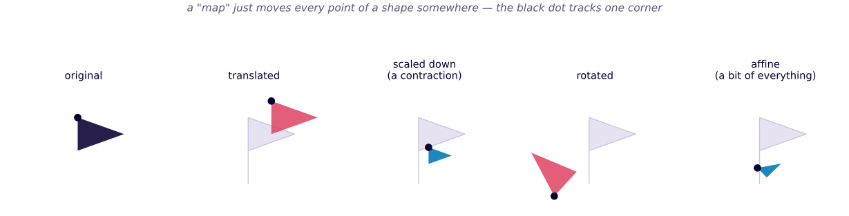
The same flag shape under five maps. A black dot tracks one specific corner in every panel, so it’s unambiguous where each point actually went.
An Iterated Function System is a finite collection of contraction maps — maps that specifically shrink whatever you feed them, always making any two points closer together than they started (the “scaled down” panel above). Apply all maps to a starting shape and take the union of the results; repeat forever. This converges to a unique attractor , no matter what shape you started from:
An attractor is just the shape this process eventually settles into, regardless of where you begin — the same idea as water finding a drain from anywhere in a sink, or a marble released anywhere in a bowl always ending up at the bottom. Start the same three maps from a triangle, a filled square, or a random round blob, and after only a few steps every one of them is converging toward the same arrangement:
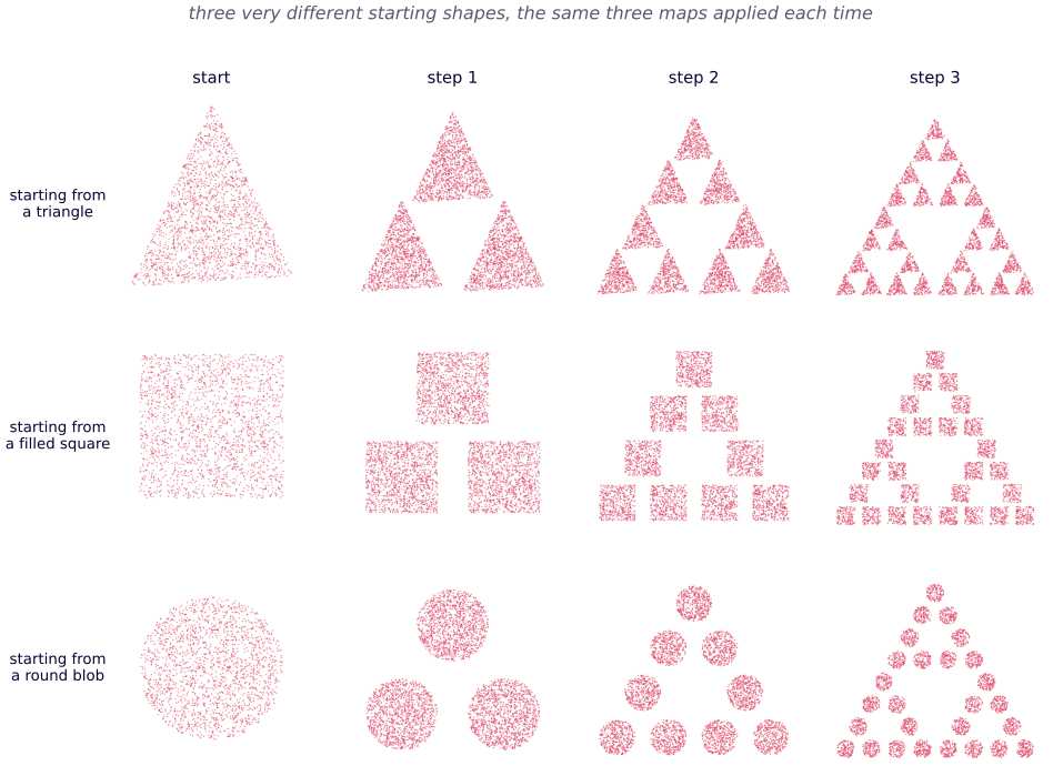
Three unrelated starting shapes, the same three maps applied each time. By step 3 the starting shape has been almost entirely forgotten — only the attractor’s own arrangement remains. This is what “attractor” means: not one particular fractal picture, but the destination every starting shape is pulled toward.
Formally:
The name is literal: you iterate a system of functions. The figure below shows one application of three simple contraction maps to a filled triangle — each map shrinks the triangle to half size and places it in a different corner. Do this once and you get three small triangles. Do it forever and you get the Sierpinski triangle.
def build(p1, p2, depth):
    if depth == 0:
        return [p1, p2]
    mid1, mid2 = split_rule(p1, p2)     # where the contraction maps send p1, p2
    return (build(p1, mid1, depth - 1)[:-1]
            + build(mid1, mid2, depth - 1)[:-1]
            + build(mid2, p2, depth - 1))
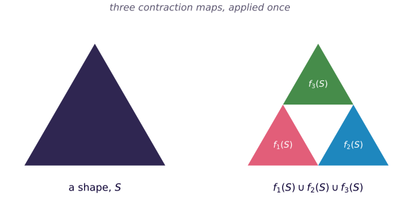
Figure: Iterate this forever and the result converges to the Sierpinski triangle, regardless of the shape you started with.
The Cantor set, Sierpinski triangle, Koch snowflake, dragon curve, and Barnsley fern are all IFS attractors.
L-systems
An L-system (Lindenmayer system) is a string-rewriting grammar: an alphabet, a starting string (the axiom), and production rules that replace each symbol with a longer string, applied simultaneously to every symbol, generation after generation — the same “simultaneous replacement” idea an IFS uses, just written on text instead of geometry. Once the string is expanded, a turtle reads it left to right and draws: move forward, turn left or right, or (for branching shapes) push and pop its position.
def rewrite(axiom, rules, iterations):
    s = axiom
    for _ in range(iterations):
        s = "".join(rules.get(ch, ch) for ch in s)
    return s

def turtle_segments(instructions, angle, step=1.0):
    # F draws forward; +/- turn; [/] push/pop (pos, heading) for branches
    ...
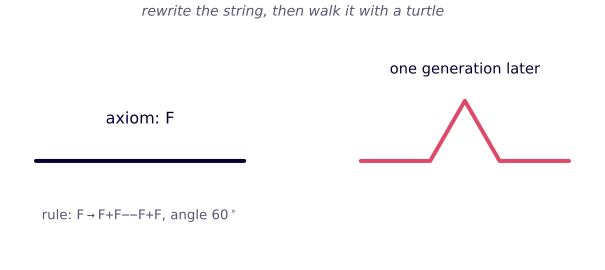
Figure: The axiom F (a single segment), and the result of applying the rule F → F+F--F+F once. Apply it forever and you get the Koch curve.
One engine, wildly different pictures, depending only on the axiom and rules you supply: a branching plant with one rule set, a space-filling curve with another.
Escape-time iteration
An escape-time fractal lives in the complex plane. For every point (either a starting value , or a parameter , depending on the fractal), iterate a fixed formula — almost always — and ask: does the resulting sequence, or orbit, stay bounded forever, or does it eventually escape to infinity? Colour each point by the answer, and the boundary between “stays” and “escapes” is a fractal. The name describes exactly this: you are timing how fast an orbit escapes.
z = np.zeros_like(c)
div_time = np.zeros(c.shape)
mask = np.ones(c.shape, dtype=bool)
for i in range(max_iter):
    z[mask] = z[mask] ** 2 + c[mask]
    diverged = np.abs(z) > 2
    div_time[diverged & mask] = i
    mask &= ~diverged
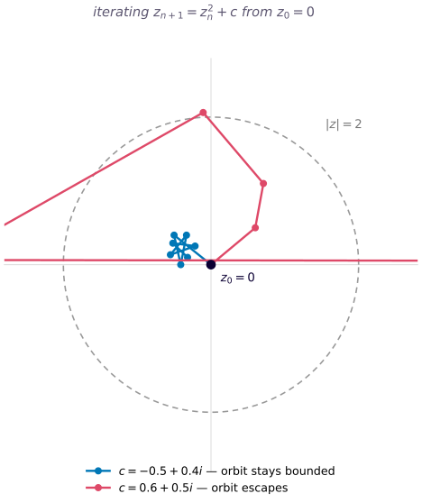
Figure: Two orbits of . Whether an orbit stays bounded or crosses and escapes is exactly the test every escape-time renderer on this site performs, once per pixel.
The Newton, Julia, and Mandelbrot sets are all escape-time fractals; only the formula being iterated, and which variable is held fixed, differs between them.
That’s the whole toolkit. Every chapter from here on names one specific fractal, gives its history and defining equation, and shows the Python (and Haskell) code that draws it — start with the Cantor Set, the simplest one in the book.