Julia Sets · Fractal Fair

Fix the parameter, vary the starting point — the mirror image of the Mandelbrot construction next door.

LINKED EXPLORER

Mandelbrot chooses the parameter; Julia reveals its world

Click anywhere in the Mandelbrot plane. That point becomes c in z ← z² + c, and the Julia set on the right is redrawn immediately.

Mandelbrot planeclick to choose c

Julia set J_cc = −0.800 + 0.156i

Same formula, different question: Mandelbrot varies c; Julia fixes c and varies z₀.

History

Gaston Julia and Pierre Fatou independently developed the theory of iterated rational functions during the First World War — Julia famously working in part from a hospital bed, publishing his 268-page memoir on iteration in 1918. The subject then fell into relative obscurity for over fifty years, lacking any way to actually visualise what Julia and Fatou could only describe with theorems.

Anecdote

Julia’s 268-page memoir was, remarkably, largely complete before computers existed to draw a single one of the sets it describes — pure analysis, verified visually only decades later.

Construction

z_{n+1} = z_n^2 + c

Exactly the same escape-time test used for the Mandelbrot set, with one difference: here $c$ is fixed and $z_0$ varies over the plane (for Mandelbrot, $z_0=0$ is fixed and $c$ varies). This single swap is why the two chapters share almost identical code — and it changes what the picture means: a Mandelbrot pixel asks “is this $c$ well-behaved?”, while a Julia pixel asks “is this starting point well-behaved, for one fixed $c$ ?”

A quick worked example with this chapter’s own $c = -0.7 + 0.27015i$ , starting from $z_0 = 0.1$ : $z_1 = 0.1^2 + c = -0.690 + 0.270i$ ; squaring and adding $c$ again gives $z_2 \approx -0.297 - 0.103i$ ; five iterations in, $|z_5|\approx 0.67$ — still comfortably inside $|z|<2$ , so this particular $z_0$ turns out to belong to the set. Nudge $z_0$ just slightly and the same handful of steps can send the orbit past $|z|=2$ and off to infinity instead; the boundary between the two behaviours is the fractal in the figure below.

★Cool Fact

The parameter used here, $c = -0.7 + 0.27015i$ , sits in a thin filamentary region of the Mandelbrot set and produces one of the most famous “dendrite-adjacent” Julia sets — delicate, spiral, and connected, but only just.

Python implementation

Pseudocode first

Algorithm in one glance Escape-time

Fix c, vary the starting point

for each pixel z0 {
    z = z0
    repeat until |z| > 2 or the limit is reached
        z = z*z + c
    colour by escape time
}

The executable version keeps the same shape; shared plotting/export details live in fractalfair_helpers.py.

z = grid_of_starting_points()
for i in range(max_iter):
    z[alive] = z[alive]**2 + c
    escaped = alive & (abs(z) > 2)
    time[escaped] = i + 1
    alive &= ~escaped

λThe Same Idea in Haskell

c :: Complex Double
c = (-0.7) :+ 0.27015

escapeTime maxIter z0 = go 0 z0
  where
    go n z | n >= maxIter    = 0
           | magnitude z > 2 = fromIntegral n / fromIntegral maxIter
           | otherwise       = go (n+1) (z*z + c)

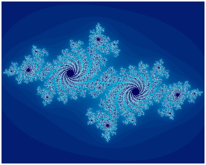
Julia set — **Figure:** Coloured by smoothed escape time on an ocean palette. The single connected filigree structure is characteristic of parameters drawn from a thin filament of the Mandelbrot set.