The Hilbert Curve · Fractal Fair

A cleaner space-filling curve than Peano's, and — unlike Peano's — one with real engineering applications.

History

A year after Peano’s shockwave, David Hilbert gave a cleaner, more geometric construction, published in 1891. Where Peano subdivides each cell into a 3×3 grid, Hilbert’s subdivides into 2×2 — a simpler picture that Hilbert, unlike Peano, actually drew.

Anecdote

Hilbert was, by the 1890s, already one of the most influential mathematicians alive — he would go on, in 1900, to pose the 23 problems that shaped twentieth-century mathematics. His space-filling curve paper is barely two pages long.

Construction

Like every curve in the L-Systems chapter, this one comes from an axiom and a pair of rules, rewritten generation after generation and handed to a turtle. Before looking at the rules themselves, it’s worth watching what the very first rewrite actually draws.

Applying rule $A$ just once to the axiom A gives the string -BF+AFA+FB-. The turtle only responds to F, +, and - — the As and Bs inside it are placeholders for what happens on the next rewrite, not drawing instructions — so walking this string means: turn right, forward, turn left, forward, turn left, forward, turn right. Three segments, a simple “U”:

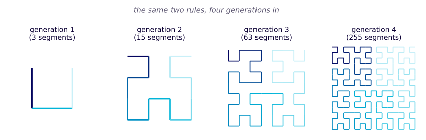
Generations 1 through 4 of the Hilbert curve build-up — The same two rules, four generations in. Each generation replaces every `A` and `B` with a slightly rotated, slightly reflected copy of the whole pattern — by generation 4, the individual U-shapes have already dissolved into the familiar dense curve.

Now the full rule set — the one every one of those generations actually used:

A \to {-}BF{+}AFA{+}FB{-}, \qquad B \to {+}AF{-}BFB{-}FA{+}

Each step multiplies the segment count by $4=2^2$ : $D = \log 4/\log 2 = 2$ . Unlike Peano’s curve, the Hilbert curve never revisits a point, and its quadrant ordering gives unusually strong locality: nearby points along the curve stay nearby in the plane.

★Cool Fact

Locality — not just space-filling — is what makes Hilbert’s curve special. Two points close together along its 1-D parameter are, with high probability, also close together in 2-D. This holds far better for Hilbert’s ordering than for Peano’s or a naive row-by-row scan.

Python implementation

Pseudocode first

Algorithm in one glance Rewrite

Change the grammar, not the engine

hilbert(n) {
    word = rewrite("A", HILBERT_RULES, n)
    return turtle(word, angle=90)
}

The executable version keeps the same shape; shared plotting/export details live in fractalfair_helpers.py.

def hilbert(iterations=5):
    word = rewrite(AXIOM, RULES, iterations)
    return np.array(turtle_segments(word, 90))

λThe Same Idea in Haskell

rules = M.fromList
  [ ('A', "-BF+AFA+FB-")
  , ('B', "+AF-BFB-FA+") ]

main = mainWith (hilbertDiagram 5 # centerXY # frame 0.05)

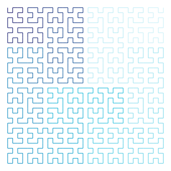
Order-5 Hilbert curve — **Figure:** 1023 segments visiting all 1024 cells of a 32×32 grid without ever crossing itself.

Where You've Seen This

The Hilbert curve’s locality underlies real spatial-indexing systems (Uber’s H3, Google’s S2), improves cache-hit rates when traversing large 2-D/3-D arrays, and appears in colour-quantisation and IP-address visualisation tools.